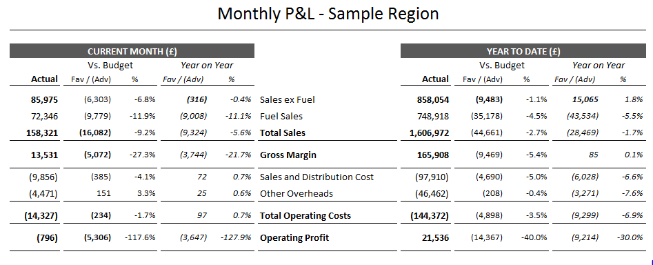
In an Excel management accounts report I was asked to include a table of KPIs below a summary P&L. The P&L had sections for current month and year to date, and displayed variances to budget and last year.

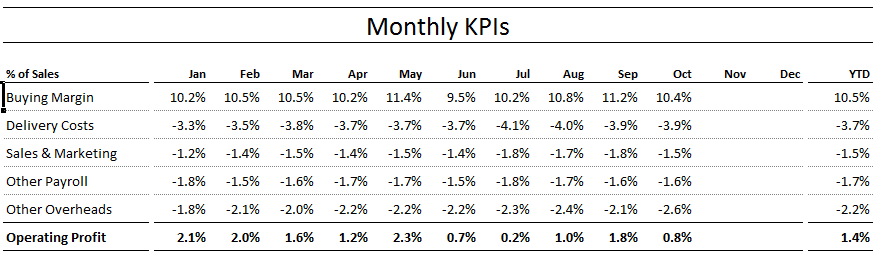
The two tables are shown below - they have a similar number of columns but with very different widths. Excel's brilliant Camera tool helped me to show both tables on one page without affecting all of the column widths or having to spend ages merging columns.

How It Works

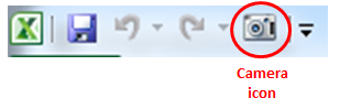
Camera lets you take a picture of one area of a spreadsheet and display it in another area - even on a different worksheet. The picture is dynamic, so if the source area changes then so will the picture.

Using Camera

1. Make sure that the Camera icon is on a toolbar. I have this icon on my Quick Access Toolbar!
2. Create the table you want to take a picture of. I recommend doing this in a separate worksheet.
3. Select the cells that you wish to copy
4. Click on the Camera icon and then click on the worksheet where you want to display the picture.

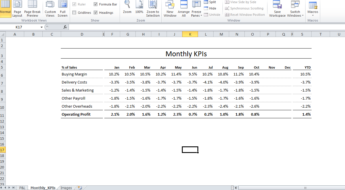
You have now created a dynamic image - this can be dragged to the required location, re-sized and formatted in the same way as any other image.