
Spreadsheets for financial and other reporting usually accumulate rows during the year. Each week or month, another set of source data rows is added to the data sheets.
A great design principle to follow is that your workings sheets should not need updating from one week or month to the next. But if the number of rows keeps changing, how can your formulas handle this?
Suppose you want to add up all the values in a column of sales data to get year-to-date sales across every location or product. A commonly used option is to sum the whole column using: =SUM($B:$B)
This does work and the formula won't need to be updated ... but this is an efficient formula as each of the 1,048,576 cells in the column will be evaluated. This increases file size and processing time, significantly in the case of larger files.
Choose a range size that you think will not be exceeded - for example =SUM($B1:$B100000).
This still has the downside of evaluating empty cells, and creates an ongoing need to check that your 'arbitrary' limit has not been exceeded.
Dynamic ranges automatically re-size when rows are added to or deleted from a range. They use Excel's OFFSET function.
= OFFSET ( reference, rows, cols, [height], [width] )
The OFFSET function has three mandatory inputs: reference, rows and cols. The following diagram shows how they work together:
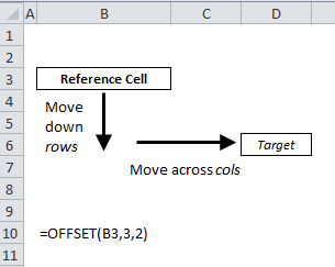
The OFFSET function is used in cell B10. The first input, reference, is of another cell - in this case B3, labelled as 'Reference Cell'.
The function then moves to a Target cell, in this case D6. This target cell is reached by moving down 3 rows and across 2 columns - based on the rows and cols inputs in B10.
The basic OFFSET function in B10 would therefore return the value of D6.
But OFFSET can be more advanced than this if the two optional inputs [height] and [width] are used.
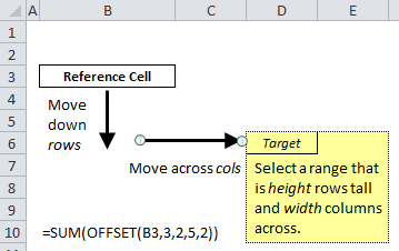
In the diagram above, the amended formula in B10 has a [height] value of 5 and a [width] value of 2. So, the function moves to the target cell (D6) as before but then selects a 5x2 block with D6 in the top-left corner (D6:E10).
In this examples, the OFFSET function is wrapped in a SUM function, so B10 would evaluate the sum of the range D6:E10.
We now know that OFFSET can have five inputs - and any of these can themselves refer to other cells. In the example below rows will be added each month. The reference cell is the column header (B3). The target cell is the first with data in (B4). To get from B3 to B4 means moving down 1 row and across 0 columns. So the rows input is 1 and the cols input is 0.
The [height] is variable and the [width] is 1, as we are only looking at one column.
Height is calculated in cell D8 using the COUNTA function - this counts the number of non-blank cells in a range. Here the range is the entire column - note the -1 which deducts the column heading from the total.
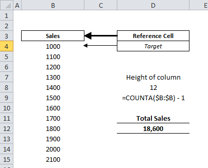
The total value of sales in column B can now be calculated using the formula in D12, as shown above. This uses the height formula in D8. Adding a value to the list in column B will update both the height value in D8 and the sales total in D12.
The best workings sections within spreadsheets shouldn't need to be updated.
Dynamic ranges are a great way to help achieve this and reduce the day-to-day admin that your spreadsheets need.